What this is. An explainer and my take on TurboQuant, a vector quantization method from Google Research (ICLR 2026). I did not write TurboQuant. The paper has the real algorithm and the proofs. The NumPy below is illustrative: small toys that build the intuition for each idea, not the method itself. I ran every snippet; the numbers are real.
The thing nobody quantizes: the overhead
When people say “we quantized the model to 4 bits,” they usually mean the weights, or in long-context inference, the KV cache. The pitch is simple: store each number in 4 bits instead of 16 or 32, get a 4x to 8x memory cut, serve longer contexts or bigger indexes on the same hardware.
The catch is that you cannot quantize a vector with just the quantized values. You also need the constants that say how to decode them, typically a scale and a zero-point per group of values, and those are usually kept in full or half precision. That bookkeeping is real memory, and it is charged against your compression budget. Watch what it does to a nominal “4-bit” scheme:
# 4-bit values, with an fp16 scale + zero-point stored per group of size G
for G in (32, 64, 128):
    overhead = 2 * 16 / G          # two fp16 constants, amortized per value
    print(f"group={G:3d}: {4 + overhead:.2f} bits/value (+{overhead/4*100:.0f}%)")
group= 32: 5.00 bits/value (+25%)
group= 64: 4.50 bits/value (+12%)
group=128: 4.25 bits/value (+6%)
Your “4-bit” cache is 4.25 to 5 bits once you count the constants. Use smaller groups for better accuracy and the overhead grows; use larger groups to shrink overhead and accuracy suffers. At 3-bit targets the tax is proportionally worse. This is the problem TurboQuant goes after. Its headline is not a fancier quantizer. It is a quantizer that needs almost no constants, and a residual step that needs none at all.
Idea 1: random rotation makes any vector boring
Quantizers love well-behaved data: values spread smoothly, no wild outliers, the same shape in every direction. Real activations and embeddings are not like that. They are spiky and anisotropic, with a few huge components that force a large scale and waste resolution on everything else.
There is a beautiful, almost unfair fix: multiply the vector by a random orthogonal matrix. Rotation preserves lengths and dot products, so it changes nothing that matters for retrieval, but in high dimensions it smears any vector into something that looks Gaussian and isotropic.
import numpy as np
rng = np.random.default_rng(0)
def kurt(x):
    x = x - x.mean()
    return np.mean(x**4) / (np.mean(x**2)**2) - 3   # 0 for a Gaussian

d = 4096
x = np.zeros(d); x[rng.choice(d, 20, replace=False)] = rng.normal(0, 8, 20)  # spiky
Q, _ = np.linalg.qr(rng.normal(size=(d, d)))                                  # random rotation
xr = Q @ x

print(f"before: kurtosis={kurt(x):7.1f}  max/std={np.abs(x).max()/x.std():5.2f}")
print(f"after : kurtosis={kurt(xr):7.2f}  max/std={np.abs(xr).max()/xr.std():5.2f}")
before: kurtosis=  713.0  max/std=38.23
after : kurtosis=   -0.01  max/std= 4.05
A vector with kurtosis 713 and a component 38 standard deviations out becomes, after one rotation, indistinguishable from Gaussian noise with a tame 4-sigma maximum. That is the whole basis for data-oblivious quantization. You do not need to study your dataset, build a codebook, or tune anything, because after the rotation every dataset looks the same. One fixed scheme, calibrated to a Gaussian, works for all of them. (In practice you use a structured rotation like a random Hadamard transform so it costs O(d log d) instead of O(d^2), but the QR rotation above shows the effect honestly.)
Idea 2: PolarQuant, or how to stop storing constants
Once your vector is isotropic, TurboQuant’s first stage, PolarQuant, leans into the geometry. Instead of quantizing Cartesian components independently, each needing its own scale, it represents the vector in polar form: a magnitude (radius) and a set of angles (direction). After the random rotation the angles are not arbitrary; they follow a known, concentrated distribution. Because the distribution is known ahead of time, you do not need to store per-vector normalization constants to decode the angles. You quantize the radius once and the angles against a fixed, pre-agreed grid.
That is the move that kills the overhead from the first section. The constants that cost you 0.25 to 1 extra bit per value mostly go away, because the rotation made their values predictable instead of data-dependent. You get high-quality 3-to-4-bit quantization with almost no bookkeeping, and crucially with no training and no calibration pass.
Idea 3: QJL, error correction in a single bit
PolarQuant leaves a small residual error. TurboQuant’s second stage, QJL (a quantized Johnson-Lindenstrauss transform), cleans it up using the cheapest unit of information there is: one sign bit per projection, with zero stored constants.
Why does a pile of sign bits carry geometry at all? Project two vectors onto a random direction and look only at the signs of the results. The probability that the signs disagree is exactly the angle between the vectors divided by pi. So if you keep many random sign bits, the fraction that disagree estimates the angle, and therefore the dot product, with no magnitudes stored at all. This is the SimHash result, and it is the intuition behind QJL:
def cos(a, b): return a @ b / (np.linalg.norm(a) * np.linalg.norm(b))

d = 4096
for bits in (64, 256, 1024, 4096):
    errs = []
    for _ in range(200):
        a = rng.normal(size=d); b = rng.normal(size=d)
        R = rng.normal(size=(bits, d))
        sa, sb = np.sign(R @ a), np.sign(R @ b)   # 1 bit per projection
        disagree = np.mean(sa != sb)
        cos_est = np.cos(np.pi * disagree)        # recover cosine from sign bits
        errs.append(abs(cos_est - cos(a, b)))
    print(f"bits={bits:5d}: mean cosine error {np.mean(errs):.4f}")
bits=   64: mean cosine error 0.1455
bits=  256: mean cosine error 0.0816
bits= 1024: mean cosine error 0.0421
bits= 4096: mean cosine error 0.0200
Pure sign bits, nothing else stored, and the cosine comes back. The error falls like 1 over the square root of the bit count, halving every time the budget quadruples, exactly as the theory predicts. TurboQuant applies this not to the raw vector but to the tiny residual PolarQuant leaves behind, so a handful of zero-overhead sign bits corrects most of the remaining error. Rotation plus polar coding plus sign-bit residual is the whole pipeline.
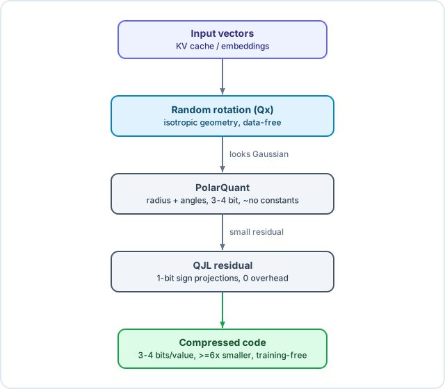
The two-stage pipeline: randomize the geometry, quantize the now-predictable polar form with almost no constants, then correct the residual with zero-overhead sign bits.
Why this matters
Two payoffs fall out of “data-free and overhead-free,” and they land on two very different systems.
LLM inference. The KV cache is the memory wall for long context. TurboQuant reports at least 6x KV-cache compression at 3-to-4 bits with no fine-tuning, and up to 8x throughput over fp32 keys on an H100, while holding accuracy across long-context suites like LongBench, RULER, and Needle-in-a-Haystack. No calibration data, no retraining, drop it in.
Vector search. The same method compresses embeddings for retrieval, and the blog reports it beating codebook methods like PQ and RaBitQ on recall, despite those methods using large learned codebooks and dataset-specific tuning. That is the part I find genuinely surprising, and it is the heart of my take.
My take: data-free should not win, and that is the point
The intuitive bet is that a method which studies your data should beat one that ignores it. A learned codebook can mold itself to the actual distribution of your embeddings; a data-oblivious scheme cannot. So “data-free matches or beats tuned codebooks” sounds like it should be impossible.
The reconciliation is the rotation. By randomizing the geometry first, TurboQuant removes the very structure a codebook would exploit, and replaces it with structure it can prove things about. You trade “adapt to this dataset” for “make every dataset identical, then be optimal for that one shape.” When the optimum for the canonical shape is near the information-theoretic floor, there is little left for a tuned codebook to win back. That is why the paper can talk about operating near theoretical lower bounds rather than just benchmark wins.
For practitioners the implication is the boring-in-a-good-way kind: fewer moving parts. No calibration set to assemble, curate, and worry about drifting. No per-dataset retraining when your corpus changes. No codebook to ship, version, and keep in sync. The cost moves to a fixed rotation you apply at write and query time, which is cheap with a structured transform.
What I would check before betting on it
- The rotation is not free at scale. A naive dense rotation is O(d^2). The structured transforms that make it O(d log d) are the difference between practical and not, so I would benchmark that path on my own dimensions, not assume it.
- Reproduce the recall on my vectors. “Beats PQ and RaBitQ” is a claim about specific datasets (GloVe at d=200, among others). Embedding distributions vary; I would rerun the recall comparison on my real corpus before retiring a tuned index.
- Where it does not apply. This compresses vectors: KV caches, embeddings. It is not a weight-quantization story for the matmuls themselves, and the accuracy claims are about retrieval and long-context behavior, which is not the same as every downstream task.
None of that dims the core idea, which is genuinely elegant: the cheapest thing to store is the thing you arranged not to need. If you want the real algorithm, the proofs, and the full benchmarks, read the Google Research writeup. The toys above are just here to make the intuition click.